How to Add Custom Fields to Pivot Tables: Easy Steps & Examples

Pivot tables are already pretty good at turning spreadsheet chaos into something you can actually use. But sometimes “Sum of Sales” and “Count of Orders” just do not cut it. You need profit margin, average order value, bonus payout, conversion rate, or some other made-up-on-purpose metric that tells the real story. That is where custom fields come in.

If you have ever stared at a pivot table and thought, “This is helpful, but not helpful enough,” you are in the right place. Adding custom fields to pivot tables lets you create your own calculations without rewriting the original data. In Excel, these are usually called calculated fields. In other spreadsheet tools, you may see similar language like custom calculations or calculated fields in the pivot editor.

In this guide, you will learn what custom fields are, when to use them, how to add them step by step, and which mistakes make people question their life choices at 4:57 p.m. on a Friday. You will also get practical examples you can steal immediately for reports, dashboards, and everyday spreadsheet survival.

What Are Custom Fields in a Pivot Table?

A custom field in a pivot table is a calculation you create using the fields already in your source data. Instead of editing the dataset itself, you add a new formula inside the pivot table so it can return a fresh metric such as profit, markup, margin percentage, or revenue per unit.

Think of it as adding a virtual column without touching the original table. That is handy when the source data comes from another team, a live export, or a file you absolutely should not “clean up” by hand unless you enjoy awkward Slack messages.

For example, if your data includes Sales and Cost, you can create a custom field called Profit with a formula like =Sales-Cost. If your data includes Orders and Revenue, you can create Average Order Value with =Revenue/Orders.

Before You Add a Custom Field, Set Yourself Up for Success

Before diving into menus, make sure your source data is pivot-friendly. Pivot tables love clean, boring, well-behaved data. If your spreadsheet is dramatic, the pivot table will be dramatic too.

Use a flat data table

Your source should have one row per record and one header per column. Avoid merged cells, blank header names, extra subtotal rows, and artistic spacing that makes the sheet look “nicer” but breaks everything later.

Make sure numeric fields are truly numeric

If your Sales column contains dollar signs typed as text, or your Quantity column contains a random “N/A” wedged between numbers, your custom field may return nonsense or fail altogether.

Know whether you are using a classic PivotTable or a Data Model PivotTable

This matters a lot. In classic Excel PivotTables, you can add calculated fields directly through the ribbon. In Data Model or Power Pivot-based PivotTables, that option may not appear because those models use measures instead. If you open the pivot and the calculated field option seems to have vanished into the void, this is usually why.

How to Add Custom Fields to Pivot Tables in Excel

Here is the straightforward process for adding a custom field to a standard Excel PivotTable.

Step 1: Build your pivot table first

Select your source data, go to Insert > PivotTable, and place the pivot table in a new or existing worksheet. Add the row, column, and value fields you need so the basic summary is already in place.

Step 2: Click anywhere inside the pivot table

This activates the PivotTable tools on the ribbon. In most recent Excel versions, you will see a PivotTable Analyze tab.

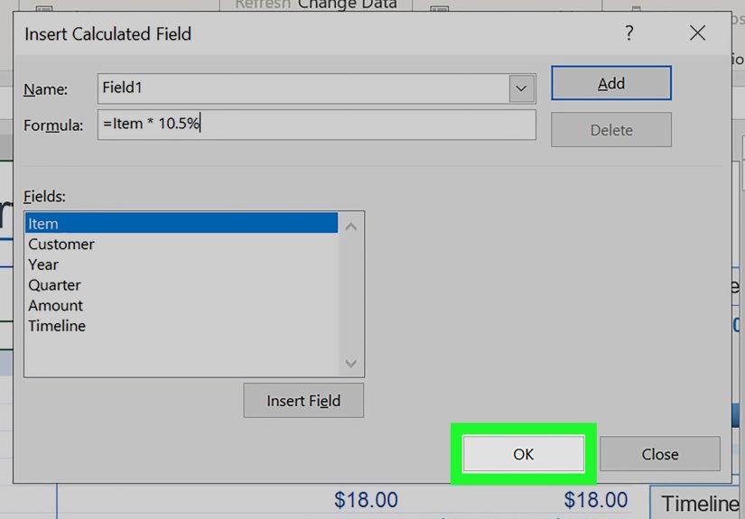
Step 3: Open the calculated field dialog

Go to PivotTable Analyze > Fields, Items & Sets > Calculated Field. This opens the Insert Calculated Field box where the custom field magic happens.

Step 4: Name your custom field clearly

In the Name box, enter something readable like Profit, Margin %, or Revenue Per Unit. This is not the time for mystery labels like Calc1_final_new2.

Step 5: Enter the formula

In the Formula box, create your calculation using field names, not cell references. That last part is important. Pivot table custom fields do not behave like regular worksheet formulas. You reference fields such as Sales, Cost, or Orders, not cells like B2 or D17.

Example formulas:

• =Sales-Cost
• =(Sales-Cost)/Sales
• =Revenue/Units
• =Sales*0.05

Step 6: Insert fields instead of typing them blind

Use the Insert Field button or double-click field names from the list when possible. It helps avoid typos, spacing mistakes, and the classic “Why is this broken?” moment caused by one missing character.

Step 7: Click Add or OK

Once the formula looks right, click Add or OK. Excel will create the new custom field and place it in the pivot field list, usually in the Values area.

Step 8: Format the result

Your shiny new field may appear as a raw decimal or overly dramatic number with twelve decimal places. Right-click the values, choose Value Field Settings or Number Format, and apply the right format such as Currency, Percentage, or Number.

Step 9: Review the results carefully

Do not assume the formula is right just because Excel did not object. Check a few totals manually. A custom field can be technically valid and still be analytically wrong for your use case.

Step 10: Edit or delete when needed

Need to fix the formula later? Go back to Fields, Items & Sets > Calculated Field, choose the existing field from the name list, then modify or delete it. Excel also lets you list formulas used in the pivot if you need a quick audit.

Easy Examples of Custom Fields You Can Use Right Away

Example 1: Profit

Let us say your source data contains these fields:

• Product
• Region
• Sales
• Cost

Create a custom field named Profit with this formula:

=Sales-Cost

This is one of the most useful beginner examples because it turns a simple sales summary into a more meaningful business report. Total sales are nice. Profit is nicer.

Example 2: Margin Percentage

If you want to see which products look amazing in gross revenue but less amazing in actual profitability, create:

=(Sales-Cost)/Sales

Then format the field as a percentage. This works well for comparing categories, regions, or sales reps.

Example 3: Revenue Per Unit

If your dataset includes Revenue and Units, create:

=Revenue/Units

This gives you a quick average selling price or revenue-per-item metric. It is especially useful in retail, inventory analysis, and product performance reports.

Example 4: Commission Estimate

If the sales team earns a flat 5% commission, create:

=Sales*0.05

Simple, clear, and immediately useful for forecasting payouts.

When a Helper Column Is Better Than a Custom Field

Here is the nuance many tutorials skip: pivot table custom fields do not always calculate the same way as a normal row-by-row formula in your dataset. In standard Excel PivotTables, calculated fields work from summarized values, not from each source row individually.

That means some calculations can produce results that look reasonable but are not mathematically ideal. Ratios, weighted averages, and conditional logic are the usual troublemakers. If your formula depends on row-level math before summarizing, the safer move is to add a helper column to the source data first and then use that field inside the pivot table.

For example, if you need a true per-transaction margin before aggregation, calculate that in the source table rather than forcing the pivot to invent it afterward.

Custom Field vs. Calculated Item vs. Show Values As

These are not the same thing, and mixing them up is one of the fastest ways to build a report that looks smart and acts strange.

Calculated field

Uses existing fields to create a new metric like profit or margin. Best for adding a new value to the pivot table.

Calculated item

Creates a custom item within an existing field. For example, you might combine two regional items into a new one. This is more specialized and can get messy fast.

Show Values As

Changes how a value is displayed, such as percentage of total, running total, or difference from previous. If you only need percent of grand total, you may not need a custom field at all. A built-in display calculation is often faster and cleaner.

Why the Calculated Field Option Might Be Missing

If you click through the ribbon and cannot find Calculated Field, do not panic and do not blame the laptop immediately.

Here are the most common reasons:

• Your pivot table is based on the Data Model or Power Pivot.
• Your data source is OLAP-based, so classic formulas are unavailable.
• You are using a spreadsheet tool where custom fields live in a different panel or under a different name.
• You are in the wrong menu because Excel likes to rename tabs just enough to keep things exciting.

In Data Model PivotTables, you typically create a measure instead of a classic calculated field. That is a different workflow and usually uses DAX formulas.

Common Mistakes to Avoid

Using cell references

Custom fields use field names, not worksheet cells. Typing =C2-D2 will not end well.

Forgetting number formatting

A correct formula can still look wrong when a percentage appears as 0.18473821 instead of 18.47%.

Assuming every ratio belongs in a calculated field

Sometimes a helper column or measure is the better tool. Not every spreadsheet problem should be solved with one more pivot trick and crossed fingers.

Using vague field names

Name your fields so future-you can understand them. Future-you is busy and already slightly annoyed.

Can You Add Custom Fields in Google Sheets Pivot Tables?

Yes. In Google Sheets, open the pivot table editor, go to the Values section, and add a Calculated field. You can also choose a custom formula in the editor. The setup is different from Excel, but the core idea is the same: create a new metric from existing pivot data without rewriting the original table.

That said, Excel still gives you more depth for advanced pivot workflows, especially when you start working with large reports, multiple calculations, Power Pivot, or reusable dashboard logic.

Best Practices for Smarter Pivot Table Custom Fields

• Keep source data clean and structured before you build the pivot.
• Use short, descriptive field names.
• Format calculated results immediately.
• Test custom fields with a few manual checks.
• Use helper columns for row-level logic.
• Use measures for Data Model PivotTables.
• Use Show Values As when you only need percentage or running-total views.

Conclusion

Learning how to add custom fields to pivot tables is one of those spreadsheet skills that pays off ridiculously fast. Once you know where the menu lives and how the formulas behave, you can turn a basic report into something far more useful without mangling the original dataset.

The big takeaway is simple: custom fields are excellent for quick, meaningful calculations like profit, commission, and revenue per unit. But they are not magic. If your math depends on row-level detail, weighted logic, or a Data Model setup, you may need a helper column or a measure instead.

Still, for everyday reporting, custom fields are one of the easiest ways to make pivot tables feel less like a summary tool and more like a decision-making tool. And once you start using them well, plain pivot tables begin to look a little underdressed.

Real-World Experiences with Custom Fields in Pivot Tables

In real reporting work, the first custom field most people build is usually something obvious like Profit. It feels great because the result appears instantly, and suddenly the pivot table is not just summarizing numbers, it is answering a business question. That early win matters. It teaches users that pivot tables do not have to be passive. They can be shaped into tools that reflect the exact way a team thinks about performance.

Then the second experience usually arrives: a formula that looks correct but gives totals that seem a little weird. This often happens with percentages and averages. Someone builds a margin field, the grand total looks off, and the room gets quiet in the most spreadsheet-specific way possible. That is the moment when users learn the difference between calculations based on summarized fields and calculations based on individual rows. It is frustrating the first time, but incredibly useful after that. Once you understand that distinction, your reports become more accurate and your troubleshooting gets much faster.

Another common experience shows up when teams inherit files from coworkers. The pivot table works, but nobody knows how it was built. A calculated field called Adjusted Rate sits in the Values area like an ancient artifact from a lost civilization. Opening the calculated field dialog or listing formulas becomes a lifesaver. Suddenly the mystery clears: the field is just =Revenue/Hours with percentage formatting, not wizardry. This is why naming and documentation matter more than people expect.

Custom fields also become especially valuable in recurring reports. Monthly sales summaries, inventory reviews, marketing performance dashboards, and service-team scorecards often use the same few calculations over and over. Once those fields are defined clearly, reporting gets faster and more consistent. Instead of rebuilding formulas on worksheets every month, teams can refresh the source data and keep moving.

There is also a practical confidence boost that comes from learning custom fields. Many spreadsheet users feel comfortable sorting and filtering but hesitate when a manager asks for a new KPI at the last minute. Knowing how to add a calculated field changes that. You can respond with “Sure, give me two minutes,” which is a much nicer sentence than “I will need to rebuild the whole report and possibly my personality.”

The most experienced spreadsheet users eventually develop a simple instinct: use custom fields for straightforward pivot-level calculations, use helper columns for row-level logic, and use measures when the model is more advanced. That instinct saves time, reduces errors, and keeps reports from becoming tangled monsters. In other words, the real experience of working with custom fields is not just learning a feature. It is learning when that feature is the right tool, when it is the wrong tool, and when it is trying very hard but still needs backup.

SEO Tags